Fundamentals · Module 1: Bias–Variance
Module 1: Predicting House Prices
In this module, you will learn about some fundamental concepts in machine learning and AI, using the task of predicting house prices as a practical example.
The general flow of this module is:
- Understanding the Concepts: Learn about linear regression, polynomial regression, and the bias-variance tradeoff.
- Training Your Model: Train a model to predict house prices based on size.
- Apply Your Model: Test your model's predictions against your own guesses in an interactive game.
- Evaluating Model Generalization: Assess how well your model performs on unseen data.
- Conclusion: Reflect on the concepts learned and their implications in real-world applications.
1. Understanding the Concepts
The Challenge: Making Accurate Predictions
In many artificial intelligence (AI) applications, from forecasting market trends to assisting in medical diagnoses, a primary objective is to build models that can make accurate predictions on new, unseen data. This module uses the task of housing price prediction — estimating a house's price based on its size — as a practical example to explore fundamental concepts in creating predictive models.
Starting Simple: Linear Regression
To begin our journey into predictive modeling, we'll start with a foundational technique called Linear Regression.
Why linear regression? It's a simple yet powerful method for understanding and modeling the relationship between a dependent variable (what we want to predict, like house price) and one or more independent variables (the features we use for prediction, like house size). Its simplicity makes it an excellent entry point for grasping core machine learning ideas, and it forms the basis for many more advanced techniques. Despite its simplicity, it can be surprisingly effective for a wide range of problems.
In its most basic form, with a single feature (e.g., house size, x) to predict a target (e.g., house price, y), the equation is:
Where:
- y is the predicted output (house price).
- x is the input feature (house size).
- w is the weight (or slope), indicating how much y changes for a one-unit change in x.
- b is the bias (or intercept), representing the predicted value of y when x is zero.
Key Terms: Both w and b are model parameters, often denoted by θ.
Model parameters are learned from the training data, which consists of pairs of known inputs and outputs.
Handling Complexity: Polynomial Regression
A straight line is often too simple for real-world data. For instance, the relationship between house size and price might not be perfectly linear; perhaps prices increase more steeply for larger houses up to a point, or show diminishing returns with size. To capture such non-linear patterns, we can extend linear regression by using a polynomial to model the relationship between the features x and output y. Instead of just x, we now also have powers of x as additional features. That is x², x³, and so on. The model then becomes:
This is a polynomial of degree n. The degree n is a crucial setting: it determines the complexity of our model.
- A low degree (e.g., n=1) results in a relatively simple, less flexible model.
- A high degree (e.g., n=10) results in a highly flexible model that can fit very intricate curves.
Note: A degree of n = 1 will result in a linear model. Linear regression is simply a special case of polynomial regression!
The Core Dilemma: The Bias-Variance Tradeoff
This ability to adjust model complexity by changing the polynomial degree brings us directly to one of the most critical concepts in machine learning and AI: the Bias-Variance Tradeoff. Choosing the "right" complexity is essential for building a model that not only learns from the data it has seen but also generalizes well to new, unseen data.
A model's total error on unseen data can be thought of as arising from three sources:
- Bias: This is error introduced by approximating a complex system with an overly simple model. High bias means the model makes strong, possibly incorrect, assumptions about the data. It fails to capture the true underlying patterns, leading to underfitting. Such a model performs poorly on both the training data and new data. Think of it as trying to draw a detailed portrait with only a thick marker.
- Variance: This is error introduced because the model tries to perfectly predict all the small fluctuations (noise) in the training data. A model with high variance pays too much attention to this noise and learns it as if it were part of the true underlying pattern. This leads to overfitting. The model might perform exceptionally well on the training data but very poorly on new, unseen data because it has essentially "memorized" the training set rather than learning the general principles. It's like a student who crams for an exam by memorizing specific questions and answers but fails when faced with slightly different ones.
- Irreducible Error: This component is due to the natural randomness or noise in the system itself or in the features we have. No matter how good our model is, we can't get rid of this error. For example, predicting where lightning will strike is inherently uncertain, no matter how sophisticated our model is.
The trade-off between bias and variance can be visualized as a curve below, where the x-axis represents model complexity (number of features) and the y-axis represents error.
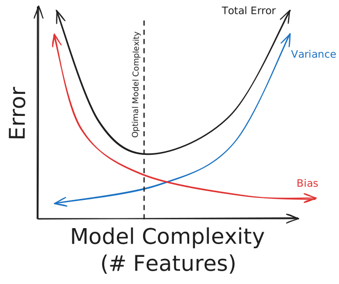
Our goal in model building is to find a sweet spot for complexity that minimizes the combined effect of bias and variance, leading to the best possible performance on unseen data. This balancing act is a central theme you'll encounter throughout your journey in AI.
2. Training Your Housing Price Model
Now that you have a basic understanding of linear regression and polynomial regression, it's time to put this knowledge into practice. In this section, you'll train a model to predict house prices based on their size.
Here you will select the housing dataset source you want to predict. There are multiple options of both synthetic and real data. For synthetic data you can also select the amount of inherent noise in the data.
After selecting the data source, you will choose how much training data you want to use to train your model as well as the polynomial degree of the model. This degree will determine the complexity of the model.
Explore different combinations of data and model complexity to see how they affect the model's performance.
The goal here is to build a model you think predicts house prices well.
Standard deviation of noise as a fraction of the true price (e.g., 0.1 = 10% noise). Set to 0 for no noise.
Controls how pronounced the curve is. Higher values create more dramatic curves.
More data can help, but real-world data is often limited or costly.
Degree of the polynomial. Higher degree means a more complex, flexible model.
Controls data generation for reproducibility.
Training Performance Metrics
3. Apply Your Model: Prediction Challenge
Now that you've trained your model, it's time to put it to the test! In this interactive game, you will predict house prices based on their size. We will present random house sizes and you will have to guess the price. You'll also see how your trained model performs on the same task. Try to outperform your model!
The game will keep track of your performance and show you how well you're doing compared to the model. Try 10–20 rounds to get a good feel for the model's performance.
🎯 Predict the price for different houses
Predict Price for House: —
Results
Overall Prediction Performance
Prediction History Table
| Size | Your Prediction | Model Prediction | True Price | Your Error | Model Error |
|---|
4. Evaluating Model Generalization
In this section, we'll do a more formal evaluation of your model's performance on unseen data. Evaluating a machine learning model on unseen data is crucial to understand how well it generalizes to new situations. This is often done using a separate test set that the model has never seen before. The test set should be representative of the data the model will encounter in the real world. In this case, we will use a separate test set of house sizes and prices to evaluate your model's performance.
The model's performance on the test set will be compared to its performance on the training set. This will help you understand how well your model generalizes to new data. Vary the amount of new, unseen data to see how the model performs. The more data you have, the better the evaluation will be.
How many new, unseen data points to use for final evaluation.
Test Performance Metrics
How did your model perform? Does it generalize well to unseen data or does it perform poorly? Can you pick out any patterns in the errors?
Consider going back and adjusting the model complexity or training data size to see how it affects the model's performance.
5. Core Ideas & Takeaways
Understanding the bias-variance tradeoff is more than an academic exercise; it's fundamental to building effective and reliable AI systems. Here are the overarching lessons from this module, with connections to broader AI challenges:
1. Model Complexity: The Double-Edged Sword of AI Power
Every AI model, from simple regression to vast neural networks, has a certain capacity or complexity. If a model is too simple for the data's inherent structure (e.g. using a linear model for a highly non-linear problem like visual object recognition), it will exhibit high bias (underfitting). It makes strong, often incorrect, assumptions and fails to learn the true patterns, leading to poor performance everywhere. This is akin to an AI that oversimplifies a complex ethical dilemma.
Conversely, if a model is too complex relative to the amount and quality of training data (e.g. an enormous language model trained on a very small, niche dataset), it can exhibit high variance (overfitting). It might "memorize" the training data, including its noise and idiosyncrasies, performing exceptionally well on it but failing catastrophically when faced with slightly new, unseen data. This lack of generalization is a major safety concern in AI, as an overfitted model might be brittle and unreliable in real-world scenarios that differ even slightly from its training conditions (i.e. out-of-distribution robustness). The quest in AI is to find models that are powerful enough to capture complex realities but are also robust generalizers.
2. Data: The Fuel and Foundation of Generalization
The characteristics of your data are paramount.
Quantity: More high-quality, representative training data generally allows for more complex models to be trained without severe overfitting. For many cutting-edge AI systems, the sheer volume of data has been a key driver of performance improvements.
Quality & Noise: The "irreducible error" reminds us that all data has limits. If data is inherently noisy or measurements are imprecise, even the best model will have some error. Understanding and quantifying this noise is crucial. In AI, this relates to data cleanliness, label accuracy, and recognizing the limitations of what can be learned from imperfect information.
Representation & Diversity: If the training data doesn't accurately represent the full spectrum of scenarios the AI will encounter in the real world, the model will likely fail when it sees underrepresented or novel inputs. This is a huge challenge in AI fairness and robustness — ensuring training data is diverse and covers edge cases. Performance on a test set is the truest measure of generalization, but even the test set must be representative of the deployment environment.
3. Navigating the Tradeoff: Practical AI Engineering
Successfully managing bias and variance involves several strategies common in AI development:
Iterative Model Selection: Start with simpler models and gradually increase complexity, always evaluating performance on a validation or test set that was not used during training. This mimics the empirical approach often taken in tuning AI architectures.
Regularization: Techniques common in machine learning (like L1/L2 penalties, or dropout in neural networks) are designed to constrain model complexity and prevent overfitting, effectively adding a bit of bias to reduce a lot of variance.
Cross-Validation: This provides a more robust estimate of how a model is likely to perform on unseen data by training and testing on multiple different subsets of the available data. It's a staple for reliable hyperparameter tuning in AI.
Domain Knowledge & Feature Engineering: Understanding the problem domain can guide the choice of appropriate model types and features, helping to inject useful "bias" that steers the model towards better solutions. In AI, this is related to choosing appropriate architectures or pre-training strategies that align with the task.
Ultimately, the "No Free Lunch" theorem in machine learning suggests that no single model or technique is universally best for all problems. The art and science of AI involve careful experimentation, rigorous evaluation, and a deep understanding of these fundamental tradeoffs to build systems that are not only accurate but also robust, reliable, and safe when deployed in the complex real world.